bomonike
 We use Python programs using Matplotlib to illustrate time and memory space complexity of algorithms (aka Big O Notation) such for sorting different ways.
![]()
![]()
![]()
![]()
![]()
![]()
![]()
![]()
![]()
![]()
![]()
![]()
![]()
Overview
Why this?
“Big O” is a set of code words about predicting what will happen when the number of elements to sort (represented by variable N) grows really big. The rhym is:
- How code slows as data grows
Symbols such as O(N^2) and O(log N) – explained in the table below – were invented in the 1970s by academics in theoretical computer scientists (such as Donald Knuth) so they (and us) can focus on each algorithm’s fundamental nature rather than implementation-specific details. See $68.66 BOOK “Introduction to Algorithms, 3rd Edition” by Thomas H. Cormen, et. al.
Now YouTuber videos say:
“If you want a job as a programmer, you need to know this”…
The assumption is that if you know the “Big-O” jargon, you also know how to use the underlying algorithms. To make that true for you, I wrote this article with the Summary Table of symbols and algorithms shown on the visualizations generated by the Python program I also wrote.
Visualizations for Sorting
Which sorting algorithm is the slowest or fastest?
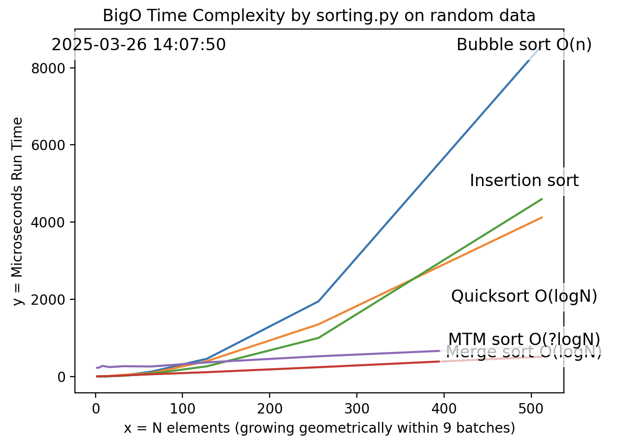
The plot above was generated by the Python program I wrote.
As the heading at the top says, the program created random values to show the worst case run times so that the most work would be needed to sort the values.
Alternately, the program can generate sequential values for sorting, which would be the best case run times because least work would be needed to sort the values.
“Big O” is the Notation about the upper-bound worst-case scenario.
There is also “Big Omega” (Ω) notation about the lower-bound best-case scenario.
There is also “Big Theta” (Θ) notation about the narrow band of an average-case scenario which is often what users experience in real-world applications. Big Theta provides a balanced and practical understanding of how algorithms perform under normal conditions.
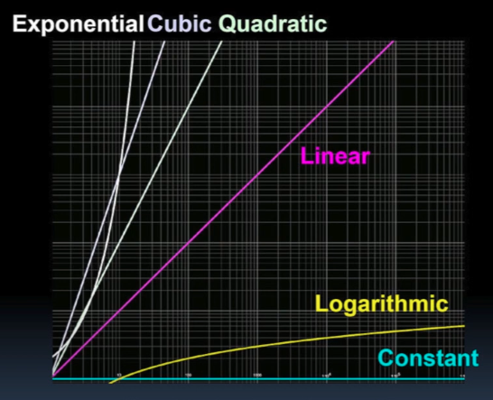
Not shown above are run times for asymptotic Exponential (Factorial), Cubic, and Quadratic algorithms.
The asymptote of a curve is a line such that the distance between the curve and the line approaches zero as one or both of the x or y coordinates tends to infinity.
Those are shown in this “log-log” plot (from BJC) of the six basic algorithmic complexity types:
Summary Table
In order of growth in the dominant term:
| Notation | Name | Usage | |
|---|---|---|---|
| O(1) | Constant (same) for all inputs n. | Access, calculation, or lookup after Memoization to/from a table (or already sorted) | |
| O(LogN) | Logarithmic | When inputs are divided in segments. No horizontal asymptope, but approaches 32 for base 2. | |
| O(N) | Linear | Bubble sort: Recalculate once for each element. | |
| asymptotic (toward infinity) | |||
| O(N^2) N squared | Quadratic | Each item looks at all other items | |
| O(N^3) N cubed | Cubic | Loop Z within loop Y within a loop X | |
| O(c^N) 2 or c to the N | Exponential | Traverse a tree with a span of 2 = c and depth of N. | |
| O(N!) | Factorial | Fibonacci recusion (gets really slow real fast) | |
Python program
https://www.programiz.com/online-compiler/2hIYYUNNRqIBp
The plot of run times for sorting was generated by my Python codecode at:
https://github.com/wilsonmar/python-samples/blob/main/sorting.py
But to experiment with a program usign only an internet browser (on a Chromebook without a local hard drive and installing an IDE such as VSCode):
- Programwiz.com VIDEO
- OnlineGDB.com
- Python Land’s online interpreter
- Replit.com
- https://www.tutorialspoint.com/online_python_compiler.php
- py3.codeskulptor.org
- https://www.scaler.com/topics/python/online-python-compiler/
- Pluralsight.com ?
- https://www.jdoodle.com/python3-programming-online/
- https://www.w3schools.com/python/trypython.asp
Google Colab:
- Open Google Colab by visiting https://colab.research.google.com
- Sign in with your Google account if you haven’t already.
- Click “GitHub”
- Copy this URL to your invisible Clipboard: https://github.com/wilsonmar/python-samples/blob/main/sorting.ipynb
-
Click on “Enter a GitHub URL …” and paste the URL. Press Enter.
FIXME: The Notebook Does Not Appear to Be Valid JSON
-
If “Release notes” appears, click the “X” to dimiss the panel.
- Run cells using Shift+Enter or the Run button in the toolbar.
TODO: Alternately:
- Go to https://repl.it
- Click “Create a new repl”
- Select “Python 3”
- Click “Create”
- Copy and paste the code from https://github.com/wilsonmar/python-samples/blob/main/sorting.py
- Click “Run”
Tutorials
There are several full tutorials available online:
-
“Sorting Algorithms” tutorial at RealPython.com in text and VIDEO is short and sweet.
-
VIDEO introduces NeetCode.com
Run Timing Code
For timing calculations, we use the timeit module containing this code:
import time
def timed_func(func_to_time):
    def timed(*args, **kwargs):
        start = time.perf_counter()
        res = func_to_time(*args, **kwargs)
        print(time.perf_counter() - start)
        return res
    return timed
The timeit module is designed to measure the execution time of small code snippets. It automatically runs the code multiple times to provide an average execution time, which helps in reducing the impact of external factors like system load.
To obtain timings for a defined function, first add a reference at the top of the custom program file:
from timing import timed_func
The Python decorator “@timed_func” is placed in front of each function so that Python knows to execute the module before the function is called.
@timed_func
def bubble_sort(items):
   ...
The decorator function return the execution time in seconds.
The above approach is not the ideal way to measure execution time, but it is simple and avoids the need to add extra lines cluttering up function code.
Bubble sort
Resources:
The “bubble” means each of the largest element “bubbles” to the top of the list in a series of swaps with adjacent items.
The Bubble Sort is simple to understand and implement.
@timed_func
def bubble_sort(items):
    for i in range(len(items)): # Iterate through whole list
        already_sorted = True # Set break condition
        for j in range(len(items) - i - 1): # Maintain a growing section of the list that is sorted
            if items[j] > items[j + 1]: # Swap out of place items.
                items[j], items[j + 1] = items[j + 1], items[j]
                already_sorted = False # Set sorted to false if we needed to swap
        if already_sorted:
            break
    return items
- Begins with an unsorted array.
- Scan through the array from left to right to find the largest element.
- Swap the largest element with the last element.
- Repeat steps 2 and 3 until the array is sorted.
- At the end of each iteration, the largest element is in its correct position.
Bubble sort is memory-efficient. It requires only a small, fixed amount of additional space regardless of the input size. So its space complexity is O(1).
The Bubble Sort is quadratic time complexity means it’s best suitable for small datasets (e.g., 10 elements) or nearly sorted data where its performance can be relatively efficient.
Bubble Sort is inefficient for large datasets.
Quick Sort
Resources VIDEO:
Quick Sort is a divide-and-conquer algorithm that works by selecting a ‘pivot’ element from the array and partitioning the other elements into two sub-arrays, according to whether they are less than or greater than the pivot. The sub-arrays are then sorted recursively.
import random

def quicksort(items):
    if (len(items) <= 1):
        return items
    pivot = random.choice(items)
    less_than_pivot = [x for x in items if x < pivot]
    equal_to_pivot = [x for x in items if x == pivot]
    greater_than_pivot = [x for x in items if x > pivot]

    # Recursively divide the list into elements greater than, less than,
    # and equal to a chose pivot, then combine the lists as below using recursion.
    return quicksort(less_than_pivot) + equal_to_pivot + quicksort(greater_than_pivot)
Insertion Sort
The algorithm is called “Insertion” because it inserts each element into its sorted place in the sorted sublist which grows to become the full list. That is slightly less work that the Bubble Sort.
The Insertion Sort is a simple sorting algorithm that builds the final sorted array (or list) one item at a time. So it is less efficient on large lists than more advanced algorithms such as quicksort, heapsort, or merge sort.
@timed_funcdef insertion_sort(items, left=0, right=None):
    if right is None: # If None, we want to sort the full list
        right = len(items) - 1
    for i in range(left + 1, right + 1): # If right is len(items) - 1, this sorts the full list.
        current_item = items[i]
        j = i - 1  # Chose the element right before the current element

        while (j >= left and current_item < items[j]): # Break when the current el is in the right place
            items[j + 1] = items[j] # Moving this item up
            j -= 1 # Traversing "leftwards" along the list

        items[j + 1] = current_item # Insert current_item into its correct spot

    return items
Explanations:
- The Insertion Sort begins with the second item.
The Insertion Sort is quadratic time complexity means it’s best suitable for small datasets (e.g., 10 elements) or nearly sorted data where its performance can be relatively efficient.
Merge Sort
Resources:
- RealPython VIDEO
- https://www.youtube.com/watch?v=TzeBrDU-JaY by mycodeschool
- https://www.youtube.com/watch?v=hPzlKHFc3Y4 “Theory” by Telusko
- https://www.youtube.com/watch?v=SHqvb69Qy70 “Code” by Telusko
O(n log(n)) performance.
def merge_sorted_lists(left, right):
    left_index, right_index = 0, 0 # Start at the beginning of both lists
    return_list = []
    while (len(return_list) < len(left) + len(right)):

        # Choose the left-most item from each list that has yet to be processed
        # If all are processed, choose an "infinite" value so we know to not consider that list.
        left_item = left[left_index] if left_index < len(left) else float('inf')
        right_item = right[right_index] if right_index < len(right) else float('inf')
        if (left_item < right_item): # Choose the smallest remaining item
            return_list.append(left_item)
            left_index += 1 # And move up in the list so we don't consider it again
        else:
            return_list.append(right_item)
            right_index += 1
    return return_list

# The actual merge sort is super simple!
def merge_sort(items):
    if (len(items) <= 1):
        return items
    midpoint = len(items) // 2
    left, right = items[:midpoint], items[midpoint:]

    # Recursively divide the list into 2, sort it, and then merge those lists
    return merge_sorted_lists(merge_sort(left), merge_sort(right))
Multi-Threaded & Multi-Processing Merge sort
How much more efficient would it be if Merge sort made use of a multi-core processor such as on macOS?
Multithreading has been known to improve performance for “I/O-bound tasks” that retrieve data from network requests, databases, and hard drives. Reading from a hard disk is 200 times slower than reading from memory. For example:
- It can take 1,000 ns (nanoseconds) to read 500KB from memory.
- It can take 2,000,000 ns to read 500KB from a hard drive.
- It can take 150,000,000 ns to go between New York City to Paris, France.
Having multiple threads allow other threads to process in the CPU while other threads are delayed waiting for I/O to complete.
Here it is not appropropriate to use Python’s asyncio built-in module for handling multiple I/O-bound tasks concurrently using cooperative coroutines separate from the OS (aka “green threads”). It’s ideal for tasks like web scraping or handling multiple network requests.
Coding using the threading built-in module:
-
from concurrent.futures import ThreadPoolExecutor is for I/O-bound tasks may not provide true parallelism because Python’s Global Interpreter Lock (GIL) ensure only one thread can execute Python bytecodes at a time, to prevent “race conditions” from occuring.
PEP703: Making the Global Interpreter Lock Optional in Python for Python 3.13
-
from concurrent.futures import ProcessPoolExecutor is for CPU-bound tasks which provides each process with its own Python interpreter and memory space, allowing true parallel execution.
import concurrent.futures
import multiprocessing
import time

def cpu_bound_task(n):
    result = 0
    for i in range(n):
        result += i
    return result

# Using concurrent.futures
def main_concurrent_futures():
    start_time = time.time()
    with concurrent.futures.ProcessPoolExecutor() as executor:
        futures = [executor.submit(cpu_bound_task, 100000000) for _ in range(4)]
        results = [future.result() for future in futures]
    end_time = time.time()
    print(f"Concurrent.futures execution time: {end_time - start_time} seconds")

# Using multiprocessing if operations are limited by what happens within its CPU:
def main_multiprocessing():
    start_time = time.time()
    with multiprocessing.Pool(processes=4) as pool:
        results = pool.map(cpu_bound_task, [100000000]*4)
    end_time = time.time()
    print(f"Multiprocessing execution time: {end_time - start_time} seconds")

if __name__ == "__main__":
    main_concurrent_futures()
    main_multiprocessing()
WARNING: The overhead of swapping threads and processes may make it less efficient than using a single thread or process.
Many use NVIDIA’s proprietary CUDA libraries to perform multiprocessing on NVIDIA GPU (Graphics Processing Unit) boards, which by design run many tasks in parallel.
Explanations:
Compiled Merge sort
From a CLI, running a Python compiler such as Numba creates thread pools for parallel execution. It works by creating an executable from Python code.
Resources:
- Using Java with Phaser
- https://medium.com/codex/this-algorithm-is-faster-than-merge-sort-12564541a425
TimSort
Explanations:
TimSort uses both insertion and merge-sort strategies to produce a stable, fast sort.
# This is a simplified TimSort (check out the real code if you're
# looking for a code analysis project).

from insertion_sort import insertion_sort
from merge_sort import merge_sorted_lists

def timsort(items):
    min_subsection_size = 32

    # Sort each subsection of size 32
    # (The real algorithm carefully chooses a subsection size for performance.)
    for i in range(0, len(items), min_subsection_size):
        insertion_sort(items, i, min((i + min_subsection_size - 1), len(items) - 1))

    # Move through the list of subsections and merge them using merge_sorted_lists
    # (Again, the real algorithm carefully chooses when to do this.)
    size = min_subsection_size
    while size < len(items):
        for start in range(0, len(items), size * 2):
            midpoint = start + size - 1
            end = min((start + size * 2 - 1), (len(items) - 1)) # arithmetic to properly index

            # Merge using merge_sorted_lists
            merged_array = merge_sorted_lists(
                items[start:midpoint + 1],
                items[midpoint + 1:end + 1])

            items[start:start + len(merged_array)] = merged_array # Insert merged array
        size *= 2 # Double the size of the merged chunks each time until it reaches the whole list

    return items
Resources
Explanations here are a conglomeration of several videos:
- By various YouTubers:
- by HackerRank (1.7M views 2018) by Gail McDowell of “Cracking the Interview” book. Says “pigeon transfer speed” is O(1)
- Fireship: in 100 seconds (550K views)
- by BroCode (348K) “How code slows as data grows”
- by TheNewBoston (1.2M views)
- Fireship: deck of cards (snarky)
- by Caleb Curry
- by Codebagel “Big O in 2 minutes”
- by Michael Sambol
- by Reducible “What Is Big O Notation?”
- by Computerphile “Getting Sorted” (British accent) shows Bubble Sort
- by Aaron Jack
-
by Tom Scott “Why My Teenage Code Was Terrible: Sorting Algorithms and Big O Notation”
- by
- by Ardens “10 FORBIDDEN Sorting Algorithms” (funny?)
-
Harvard CS50
-
Berkeley BJC Lecture 7: Algorithmic Complexity
- Khan Academy (text) covers Algorithms in detail (Binary search, Asymptotic notation, Selection sort, Insertion sort, Recursive algorithms, Towers of Hanoi, Merge sort, Quick sort, Graph representation, Breadth-first search)
Quizzes
From among https://blog.bigo.tv/en/best-apps/live-trivia-apps/
https://quizizz.com/admin/quiz/5d9ec32ddeb74c001accf87f/big-o-notation 17 questions.
https://www.101computing.net/big-o-notation-quiz/
https://www.youtube.com/watch?v=mni64IAd-_U Sorting algorithms & Big O Quiz
More
This is one of a series on AI, Machine Learning, Deep Learning, Robotics, and Analytics:
- AI Ecosystem
- Machine Learning
- Microsoft’s AI
- Microsoft’s Azure Machine Learning Algorithms
- Microsoft’s Azure Machine Learning tutorial
- Python installation
- Image Processing
- Tessaract OCR using OpenCV
- Multiple Regression calculation and visualization using Excel and Machine Learning
- Tableau Data Visualization
v015 + rhym :algorithmic-complexity.md